Motion, Depth and Object Perception

The Visual Cliff

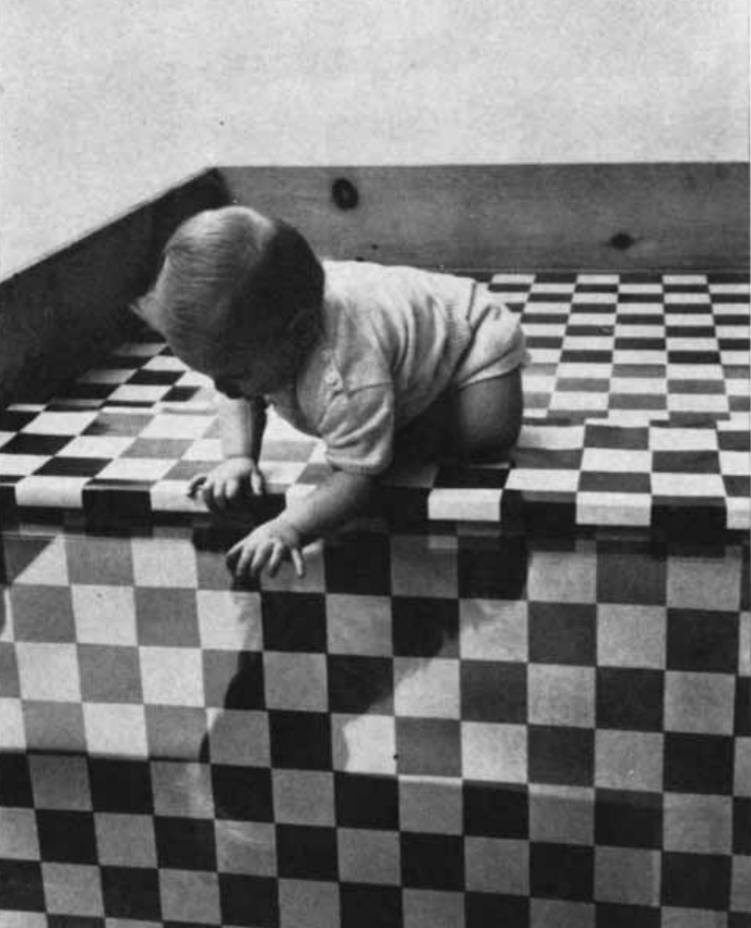
Animals learn to see without external feedback. Therefore, we should be able to program computers to do the same. Unfortunately, it is not exactly clear by which mechanism animals learn to see. In their famous paper The Visual Cliff, Gibson and Walk (1960) investigated depth perception in young rats, cats and humans. They placed a sheet of glass over a cliff and incentivized the animals to move across it.

All animals generally tended to avoid the cliff regardless of experience with cliffs or falling. The authors therefore rejected the hypothesis that depth perception is learned by trial-and-error. This, again, can make us hopeful that we might be able to avoid artificial learning agents entering situations they cannot recover from (e.g. a robot falling down a cliff).

After being able to perceive motion and depth, the notion of objects almost naturally emerges. For example, we can define objects as a set of particles that are close in space and don't disintegrate, i.e. they retain their relative position over time. Both of these notions are perfectly captured by depth and flow, which we will introduce in the following sections.

Camera Projection and Depth

First, we define a mathematical model of our camera. We use the common and simple pinhole camera model in which all rays go through a single point before being projected onto the camera sensor. Real cameras do not follow this model exactly, however, the methods described here should also apply to more complex camera models with some modifications.

As is evident from Equation (1), depth $x_3$ is lost in the projection. This makes the projection non-invertible in general. However, when we are given the depth $x_3 = D(u) \in \mathbb R$ for a pixel $u \in \mathbb R^2$, we can recover the original point $x$ as follows

This is called reprojection and trivially follows from Equation (1).

Depth can be estimated using many different signals such as object size, sharpness, occlusion. However, one of the most prominent signals is motion parallax which makes far objects appear to move across the image slower when the camera moves. In the next section we see how camera movement, apparent motion and depth are connected.

Motion Perception

Similar to how it seems to be genetically pre-programmed in some animals, motion perception can be pre-programmed in computers too. Most notable are the optical flow estimation algorithms by Lucas and Kanade (1981) and Farnebäck (2003).

Estimating motion from camera images can be challenging since cameras don't observe points directly but only the points' luminance. It might be impossible to infer from the local context whether a very smooth surface is moving or not, for example. Because of this difficulty, learned, global motion estimation has the potential to perform much better than the mentioned pre-programmed heuristics. In this section we introduce the necessary preliminaries and identities to build a self-supervised system capable of learning to estimate motion.

Scene flow is the motion of points in the scene, i.e. $S(x) = x' - x$. One of the greatest sources of scene flow is the motion of the camera itself. When the camera is rotated by $R \in \mathbb R^{3 \times 3}$ and translated by $t \in \mathbb R^3$ in an otherwise static scene we have

In general, scene flow is a combination of camera and object motion, i.e.

In the image, scene flow causes pixels to move. This is called optical flow.

In a static scene with only camera movement, optical flow $F(u) = u' - u$ can be computed by (1) reprojecting $u$ to $x$ (Eq. 2, assuming depth given), (2) applying camera motion $x' = S_\text{cam}(x) + x$ (Eq. 3), and (3) projecting $x'$ to $u'$ (Eq. 1).

This geometric constraint (among others) can be used to jointly learn to predict depth, flow and camera motion in a self-supervised manner (Chen et al., 2019).

Object Recognition via Object Tracking

Having outlined how depth, flow and camera motion can be learned in a self-supervised way, we now propose a method to use these capabilities to learn about objects. The idea is that we first learn to detect and track moving objects in a scene and then use the image sequences of the tracked objects to learn object embeddings in a self-supervised manner.

Tracking Objects

Optical flow tells us how points in a scene move in the image. This allows us to track points in the scene and also allows us to track objects as long as the pixel we are tracking stays visible and the optical flow estimation is accurate. It can happen that the tracked point becomes occluded or that the optical flow estimator points to a pixel that doesn't represent the original point anymore. This is fine if we are pointed to a new pixel that is still part of the same object. Otherwise, we need to terminate the tracking, which we discuss at the end of this section.

Initial Pixel Selection

Initial pixel selection determines which objects will be part of our generated dataset and which will not. Depending on the application, very different initial pixel selection schemes can make sense. Here, we propose two such schemes that should be general enough to be widely applied.

Random Initial Pixel. The simplest and arguably most inclusive strategy is to select random pixels in the image. This causes objects to be represented proportional to the number of pixels they occupy in the raw video data. However, this could result in tracking mostly uninteresting things such as the sky in outdoor scenes or the floor in indoor scenes. Many of these things also would not really be considered objects per se.

Moving Point Clusters. A more narrow strategy is to select a point from a moving point cluster in the scene. Here, the object distribution is heavily biased towards agents (e.g. animals, machines) and towards objects manipulated by agents (e.g. cars, tools). Since these objects are important enough to be manipulated by agents, this strategy serves as an "interestingness prior".

To detect moving points in the scene we can compute the scene flow from our depth and optical flow estimates as follows

To recover the true object movement in the scene $S_\text{obj}$ we still need to subtract the camera-induced scene flow $S_\text{cam}$:

Since $x'$ and $x$ are mapped from $u'$ and $u$, this only allows us to compute the scene flow for points that are visible in two successive images.

This filtered scene flow can then be projected back into the image giving rise to a filtered optical flow $F_\text{obj}$. Note though that the optical flow doesn't decompose as nicely as the scene flow since the camera projection is not a linear map, i.e. $F(u) \ne F_\text{obj}(u) + F_\text{cam}(u)$. Nevertheless, we can use $F_\text{obj}$ to select pixels that are due to object motion in the scene. One simple heuristic would be to blur the flow to even out small scale fluctuations and then select the pixel with the maximum flow magnitude.

Terminating Tracking

It is also important to know when to terminate tracking, e.g. when the tracked objects leave the frame or become occluded. When prematurely terminated trajectories are discarded, the termination condition can even play a filtering role.

A simple termination heuristic is to terminate whenever the combined squared difference in optical flow, depth and pixel values exceeds a certain threshold. All of these quantities should only change slowly as long as we are really tracking the same particle in the real world.

If the self-supervised encoder is trained in parallel to the trajectory generation, a more principled EM-like approach (Dempster et al., 1977) is available. Since the learned representation produced by the encoder carries information to distinguish the tracked object from others, this representation can be used as a basis for an object motion model that predicts future optical flow from past frames (and potentially future embeddings as well). This motion model can then be used in place of a hand-crafted one. In the language of EM, learning the encoder and motion model is the M-step, while selecting the correct trajectory is the E-step.

Learning from Object Trajectories

Once we have the tracking trajectories, we can split them up into separate images with the tracked pixel at the center. This is an ideal target for contrastive or Siamese learning (Grill et al., 2020; Chen and He, 2020). Instead of relying on image augmentations such as rotations or color distortions (Oord et al., 2018), the variability necessary for contrastive or Siamese learning is provided by the real world. This is a much richer form of variability since it is much more akin to what the system will later encounter during deployment in the real world. For example, we see the objects from different angles, the background varies dramatically as the objects or the camera move, and we can even learn about how objects of certain types tend to move.

Experiments

In this section we evaluate the feasibility of tracking objects with an off-the-shelf implementation of Farnebäck's dense optical flow estimator (Farnebäck, 2003) and illustrate how the tracking trajectories could then be used to generate a dataset for self-supervised learning.

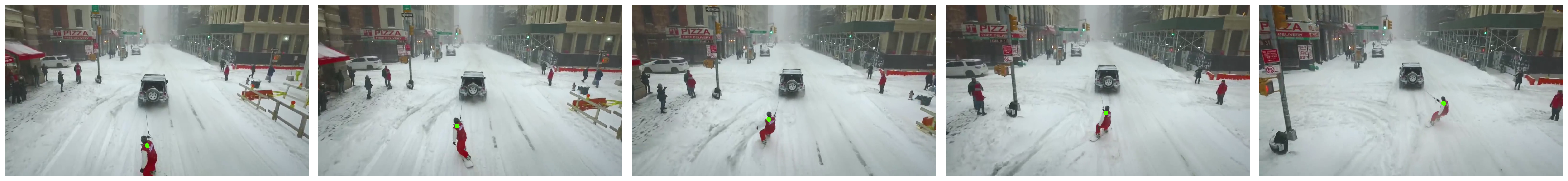
We chose a video sequence with a moving camera and moving objects (see figure above).

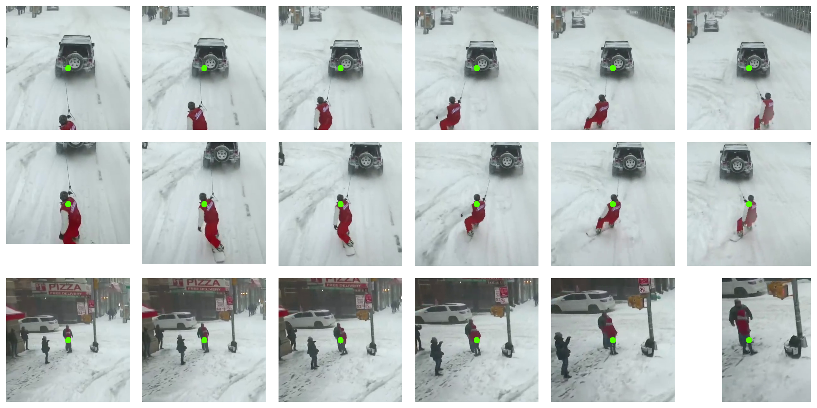
We hand-picked three initial pixels to start the tracking: (1) the car, (2) the snowboarder and (3) a pedestrian on the sidewalk. The figure above shows that it is indeed feasible to track moving objects over multiple seconds even with a traditional optical flow estimator.

It also shows the variability that can be expected from our method. Since the camera is following the car, there is little variability in the appearance of the car itself. The image sequence tracking the snowboarder shows well how different angles of the object are presented. In the case of the stationary pedestrian, the moving camera is a big source of variability and the object is presented at different distances to the camera.

References

- Chen, X. and He, K. (2020). Exploring Simple Siamese Representation Learning.
- Chen, Y., Schmid, C. and Sminchisescu, C. (2019). Self-supervised learning with geometric constraints in monocular video: Connecting flow, depth, and camera. In Proceedings of the IEEE International Conference on Computer Vision.
- Dempster, A. P., Laird, N. M. and Rubin, D. B. (1977). Maximum likelihood from incomplete data via the EM algorithm.
- Farnebäck, G. (2003). Two-frame motion estimation based on polynomial expansion. In Scandinavian Conference on Image Analysis.
- Gibson, E. J. and Walk, R. D. (1960). The "visual cliff".
- Grill, J.-B. et al. (2020). Bootstrap your own latent: A new approach to self-supervised learning.
- Lucas, B. D. and Kanade, T. (1981). An iterative image registration technique with an application to stereo vision.
- Oord, A. van den, Li, Y. and Vinyals, O. (2018). Representation learning with contrastive predictive coding.