that describe the stateful modules that make up the algorithms. Here, I want to look in detail at the mathematical assumptions that have to be made for the method to be valid. While most (but not all) of the math here can also be found scattered throughout the paper, I am trying to present it in a more linear, proof-like manner.
Why spiking neural networks?
Spiking neural networks are interesting in two ways. 1) The brain uses spikes and we want to understand how it works. 2) Spikes are binary and therefore are cheaper to communicate and store and also have the potential to reduce the costly weight multiplication in neural networks to a cheap sum of integer weights.
In the brain, each neuron has on average 7000 connections to other neurons. Therefore it makes sense to trade computation and bandwidth in the connections for computation on the neuron level, i.e. spend computation on encoding the activations.
To recap, a typical, non-spiking neural activation is computed as
x′=h(z)withz=wx=(i∑wijxi)j
where x are the activations of the previous layer (or the network inputs) and h is a non-linear function, e.g. h(z)=max(z,0).
Usually floating point numbers are used to represent weights and activations. Floating point numbers are divided into an exponent and a mantissa. To multiply them we have to integer-add the exponent and integer-multiply the mantissa. This is implemented in hardware but it still requires a lot of chip space and energy. However, if x were binary (i.e. a spike), we can compute z with a sparse sum. We could even use integers to represent w and then the multiplication would be as simple and computationally cheap as it gets.
In their paper O’Connor et al, 2018 introduce an encoding scheme that uses “integer spikes” in the forward pass, backward pass and for the weight updates without loss in accuracy compared to non-spiking networks.
One thing about the paper I found somewhat misleading is that the authors call their method spiking, when they actually use “integer spikes”. Using integers instead of binary values to communicate activations is still much cheaper than floats but it requires integer multiplications to compute the inner product with the weights. So a more appropriate name would have been “Temporally Efficient Deep Learning with Integer Activations”. Nevertheless the paper is very insightful and it would probably be possible to tweak the method in certain ways to allow it to work with only binary spikes.
Below we see the dataflow from one neuron to another neuron in a standard neural network. In the next section we will focus on the axon part, i.e., communicating the activations and trying to find a bandwidth saving encoding.
In predictive coding the sender and receiver share a model for the temporal evolution of the signal between them. Instead of communicating the original signal, only the model error is communicated and therefore only the model error is affected by channel noise which results in a higher signal-to-noise ratio.
Predictive coding is usually not used for neuron-to-neuron communication because the channel is not noisy (we usually use float32 to communicate the activations). Since we want to save bandwidth however, we will have to quantize the signal and therefore introduce quantization noise (see next section).
The neuron-to-neuron communication in a standard neural network without predictive coding can be framed as predictive coding with the model xt=0+at with the error at=xt that has to be communicated. Another very simple model would be to assume the signal stays constant, i.e. xt=xt−1+at, then we would only transmit activation changes.
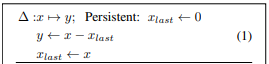
O’Connor et al. use a similar decaying model:
xt=kp+kdkdxt−1+kp+kd1at
Note that the error is at scaled by the factor kp+kd1. We can rewrite the model equation as an encoder-decoder pair:
Sigma-Delta modulation is a quantization scheme and a form of noise shaping for converting high bit-count, low frequency signals into low bit-count, high frequency signals. Let’s look at how that works:
Because quantization s=round(a) loses information, we store the “leftover”, ϕ=a−s and add it at the next timestep s=round(ϕ+a).
So, starting with ϕ0=0, we have
st=round(ϕt+at)ϕt+1=(ϕt+at)−st
Note: In general we round to the next integer. To ensure that we get binary spikes, i.e. s∈0,1 we need ϕt+at∈[0.5,1.5] and because ϕt∈[−0.5,0.5] we want at∈[0,1] which we can ensure by increasing the temporal resolution and tweaking kp and kd (see previous section).
But how can we reconstruct a from this? To get a relation between s and a we can unroll the expression for ϕt+1 for n steps
This gives us a relation between ∑a and ∑s which is a good starting point.
i=t−n+1∑tai=i=t−n+1∑tsi+ϕt+1−ϕt−n+1
To get at we have to assume at=constant over a series of timesteps t−n+1,…,t. Then, we can write
at=n1i=t−n+1∑tai=n1(i=t−n+1∑tsi+ϕt+1−ϕt−n+1)=we can accessn1i=t−n+1∑tsi+error termnϕt+1−ϕt−n+1
For n→∞ we therefore have at=limn→∞n1∑i=t−n+1tsi. Since ϕt∈[−0.5,0.5] and E[ϕt]=0 we can assume that error term is small even for small n. The scale of the sum, on the other hand, is (up to the error term) proportional to a. That means the signal-to-noise ratio of the reconstruction depends heavily on which scaling constant kp+kd1 we use for a.
Furthermore, the requirement for at to be constant across many timesteps is not a real limitation. We can just increase time resolution and increase n proportionally to make the error term small. So if x changes too quickly we can just make our timesteps smaller.
To “decode” the quantization we therefore have to average the quantized signal. Conveniently the decoding scheme from the previous section already does this implicitly (approximately):
Therefore we don’t need a decoderQ−1 for the quantization such that we end up with the following pipeline.
⟶xenc⟶Q⟶sdec⟶x^
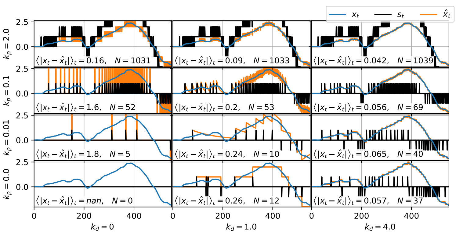
Below we can see what the combined signals look like for different encoding parameters.
Integer weight multiplication
Right now we have established more efficient communication between the neurons but still not incorporated the weight multiplication.
⋯neuron a⟶h→xenc→Qaxon⟶sQsynapsesdec→x^wQneuron b ⟶zh⋯Q(not what we want)
So we have
zt=wtx^t=wtci=0∑t(kp+kdkd)t−isi
Considering that x^t is just a weighted sum, if we assume wt=constant, we can pull it inside the sum
zt≈ci=0∑t(kp+kdkd)t−isiwt:=z^t
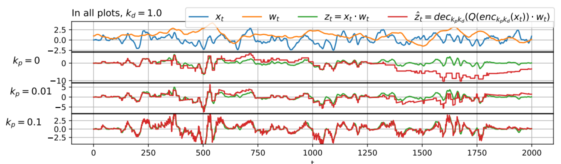
Because si is integer we have achieved our goal of replacing the floating point multiplication with a cheaper sparse integer multiplication! The approximation error we make with the assumption wt=constant depends on how fast we decay the weights inside the sum, i.e. how large kp is. Below is the final pipeline and a plot of the reconstruction for different kp.
⋯neuron a⟶h→xenc→Qaxon⟶sQsynapseswtQneuron b ⟶dec→z^h⋯Q(✓)
Learning the weights
To learn the weights we can apply the same coding scheme for backpropagation (by making the same assumptions). The symmetric backward pass through the transposed weights is not really biologically plausible but there is orthogonal work on biologically plausible backpropagation.
⋯neuron a⟶h→xenc→Qaxon⟶xˉ=sQsynapseswtQneuron b ⟶dec→z^h⋯Q(forward)⋯neuron a⟵Qh′←decaxon⟵QsynapseswTQneuron b⟵eˉQ←enc←eh′Q⟵∇x′L⋯(backward)
This leads to an efficient backward pass but in order to update the weights with gradient descent we need to compute the outer product between the activations and the next pre-activation gradients: ∇wL=x⊗e (where e=∇zL) which we both do not have access to.
The simplest solution would be to decode x^=dec(s) and e^=dec(eˉ) before the inner product.
∇wLrecon=x^⊗e^
Then we still have an expensive floating point multiplication, however. Instead we can use the fact that the result of the decoder s→dec→x^
dec:x^t=kp+kdst+kdx^t−1
decays exponentially in absence of spikes (i.e. st=0). Therefore we can calculate the sum over time between two spikes (pre-synaptic or post-synaptic) analytically as a sum over a geometric series. It is fine to sum the gradients over time and apply it as an update later, because that is what SGD does anyway.
Here, t−n is the time at which the last spike occurred. If another spike occurs for either xˉ or eˉ we just add that sum to the corresponding weight (multiplied by the learning rate). That is called “past updates” in the paper.
Summary
We looked at the forward pass, backward pass and weight updates from the paper and legitimized every step with solid math (most of which can also be found in the paper). This revealed the assumptions that had to be made and requirements on the hyperparameters as well as possible extension points to the method.