Deep Reinforcement Learning for Continuous Control
Abstract
Reinforcement learning is a mathematical framework for agents to interact intelligently with their environment. In this field, real-world control problems are particularly challenging because of the noise and the high-dimensionality of input data (e.g., visual input). In the last few years, deep neural networks have been successfully used to extract meaning from such data. Building on these advances, deep reinforcement learning achieved stunning results in the field of artificial intelligence, being able to solve complex problems like Atari games [1] and Go [2]. However, in order to apply the same methods to real-world control problems, deep reinforcement learning has to be able to deal with continuous action spaces. In this thesis, Deep Deterministic Policy Gradients, a deep reinforcement learning method for continuous control, has been implemented, evaluated and put into context to serve as a basis for further research in the field.
German abstract
Reinforcement-Learning ist ein mathematischer Rahmen, um intelligent mit ihrer Umgebung interagierende Agenten zu erzeugen. Regelungsprobleme in realen Umgebungen sind dabei wegen stark verrauschten, hochdimensionalen Eingabedaten (z.B. Video) besonders anspruchsvoll. In den letzten Jahren wurden dafür jedoch erfolgreich neuronale Netze benutzt. Deep-Reinforcement-Learning (Reinforcement-Learning mit neuronalen Netzen) hatte bereits große Erfolge in der künstlichen Intelligenz und war in der Lage komplexe Probleme wie Go [2] oder Atari-Spiele [1] zu lösen. Um diese Methoden aber in der echten Welt anwenden zu können, muss Deep-Reinforcement-Learning mit kontinuierlichen Handlungsräumen umgehen können. Deshalb wurde in dieser Thesis Deep Deterministic Policy Gradients, eine Deep-Reinforcement-Learning-Methode für kontinuierliche Regelungen implementiert, evaluiert und in Bezug zu anderen Methoden gesetzt.
Acknowledgments
I thank my supervisors Simone Parisi and Gerhard Neumann for their patience and helpful discussions, with special thanks to Simone for his support during time-critical periods.
1 Introduction
Reinforcement learning is a mathematical framework for agents to interact intelligently with their environment. Unlike supervised learning, where a system learns with the help of labeled data, reinforcement learning agents learn how to act by trial and error only receiving a reward signal from their environments. A field where reinforcement learning has been prominently successful is robotics [3]. However, real-world control problems are also particularly challenging because of the noise and high-dimensionality of input data (e.g., visual input). In recent years, in the field of supervised learning, deep neural networks have been successfully used to extract meaning from this kind of data. Building on these advances, deep reinforcement learning was used to solve complex problems like Atari games and Go. Mnih et al. [1] built a system with fixed hyperparameters able to learn to play 49 different Atari games only from raw pixel inputs. However, in order to apply the same methods to real-world control problems, deep reinforcement learning has to be able to deal with continuous action spaces. Discretizing continuous action spaces would scale poorly, since the number of discrete actions grows exponentially with the dimensionality of the action. Furthermore, having a parametrized policy can be advantageous because it can generalize in the action space. Therefore with this thesis we study a state-of-the-art deep reinforcement learning algorithm, Deep Deterministic Policy Gradients. We provide a theoretical comparison to other popular methods, an evaluation of its performance, identify its limitations and investigate future directions of research.
The remainder of the thesis is organized as follows. We start by introducing the field of interest, machine learning, focusing our attention on deep learning and reinforcement learning. We continue by describing in detail the two main algorithms, core of this study, namely Deep Q-Network (DQN) and Deep Deterministic Policy Gradients (DDPG). We then provide implementatory details of DDPG and our test environment, followed by a description of benchmark test cases. Finally, we discuss the results of our evaluation, identifying limitations of the current approach and proposing future avenues of research.
2 Foundations
Machine learning is an approach to design and optimize information processing systems by directly using data. As typically in real-world problems the training data is limited and does not cover all possible scenarios, the system has to learn how to behave also in the presence of data which it has not been trained on. In this regard, overfitting is one of the biggest challenges in machine learning and consists in having a system that strictly adapts its behavior to the training data, without being able to generalize to different unseen input data.
Machine learning is usually divided into supervised learning, reinforcement learning and unsupervised learning. Supervised learning systems learn input-output mappings from a dataset of desired input-output pairs, i.e. they are explicitly told how to behave. As we will see in the next section, most of deep learning and neural network research so far has been done in the supervised setting. Reinforcement learning systems, on the contrary, learn how to behave by receiving feedback from the environment encoding a specific goal. For example, a trash-collector robot would receive a reward for collecting trash or would be punished for hitting a wall. It is common for reinforcement learning to exploit supervised learning techniques. Unsupervised learning, on the other hand, is about finding patterns in data and will not be discussed further in this thesis. In the next sections we will describe in more detail one of the most prominent supervised learning techniques, namely deep learning and neural networks.
2.1 Deep Learning and Neural Networks
Deep learning is an area of machine learning concerned with deep neural networks. Neural networks are non-linear parametric functions loosely inspired by the human brain. They are composed of layers of units called neurons, as shown in Figure 2.1.
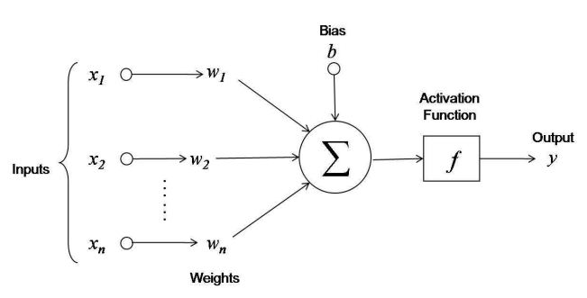
Multiple parallel neurons form a layer, each characterized by outputs called activations . Single layer (shallow) neural networks called perceptron have been first described by Rosenblatt in 1958 [4]. However in deep neural networks multiple layers are stacked on top of each other. Krizhevsky et al. [5] achieved state-of-the-art computer vision results with an 8-layer, 500,000 neurons and 60-million parameter neural network. Since the outputs of a layer are non-linear features of the input, the more layers are in the network, the more non-linear and abstract those features are compared to the original input. This hierarchy of features enables neural networks to approximate complex functions.
Neural networks are usually initialized randomly and then trained on a dataset with regard to a cost function. Typically, cost functions are distance measures between the desired outputs (targets ) and the actual network outputs (). A common and simple cost function is the mean squared error . Training a neural network consists in optimizing the network parameters to minimize the cost on the training dataset. However, training a neural network can be challenging. First, as the parameter space can be non-convex, neural networks are usually optimized with techniques guaranteeing convergence to a local optimum (e.g., gradient descent). Second, the number of parameters grows with the complexity of the network. As deep, complex networks are typically required to learn difficult functions, the training can be highly demanding, both in terms of computational time and data. Nevertheless, in practice neural networks can be optimized quite reliably by gradient descent, as we will see in the next section.
2.1.1 Stochastic Gradient Descent
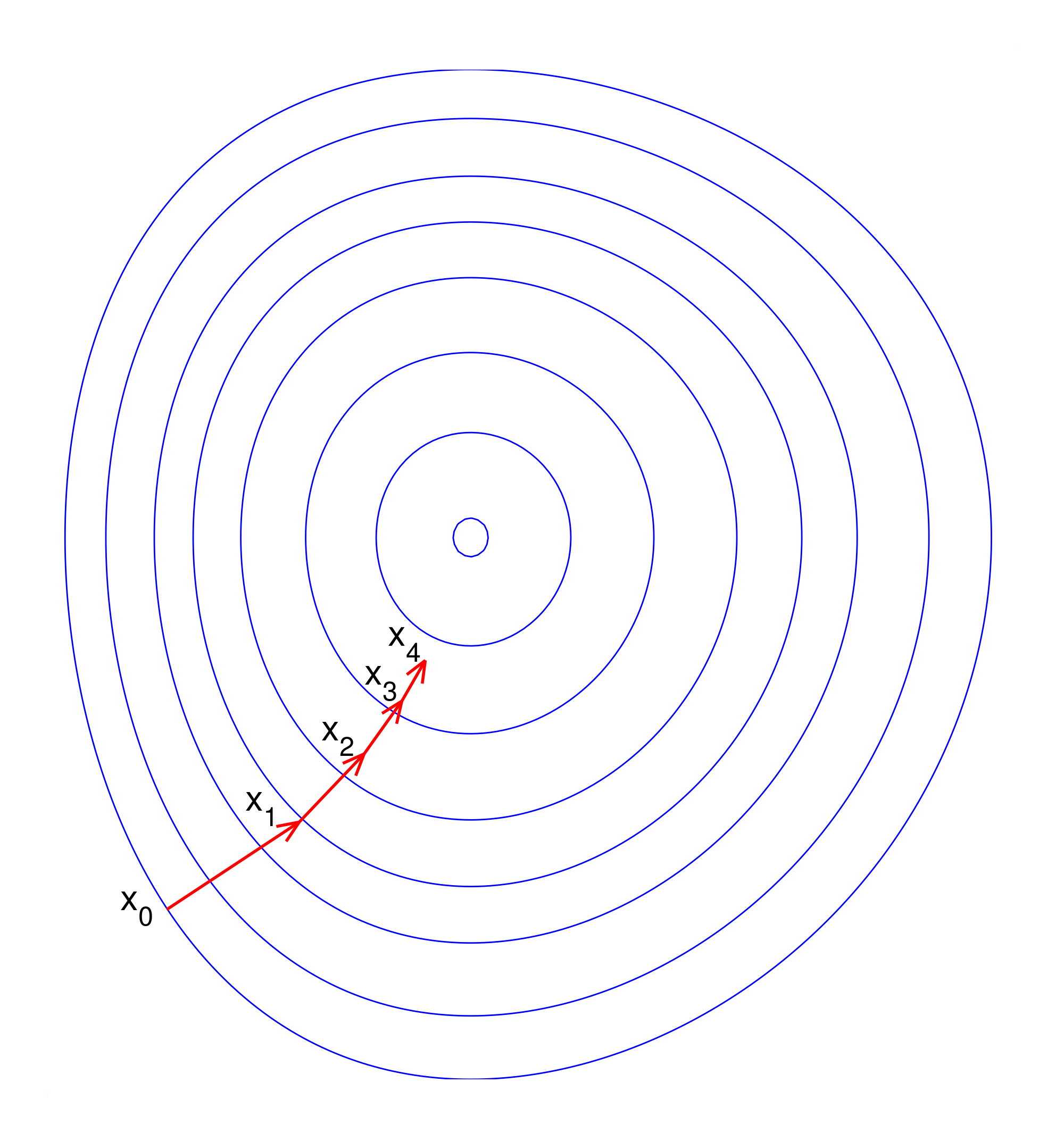
Using the gradient for optimization (i.e., first order optimization) is common to many machine learning algorithms with high number of parameters, since zeroth order methods (e.g., genetic algorithms) need several function evaluations and higher -order methods are too expensive per evaluation. Therefore, gradient descent is a key element of deep learning. It consists in following the direction pointed by the gradient of the cost function with respect to the parameters of the system. In the case of neural networks, the gradient of the cost function with respect to the network parameters tells us how to change the parameters in order to reduce the cost. More specifically, given the gradient of the cost with respect to the parameters , we can update the parameters , where is a learning rate. However, computing the cost and the gradient on large datasets is expensive. Stochastic gradient descent alleviates this issue by only computing the cost and the gradient for a small subset (minibatch) of the dataset. Like gradient descent, stochastic gradient descent is guaranteed to converge to a local minimum.
In high-dimensional optimization spaces like those of neural networks, optimization often gets stuck near saddle points or valleys where gradients are only high in directions orthogonal to the valley in which no progress can be made. This issue can be alleviated by having adaptive learning rates for each parameter. A recent version of stochastic gradient descent using these techniques and used in this thesis is ADAM [6]. Another interesting property of ADAM is that its stepsize is independent of the scale of the gradients.
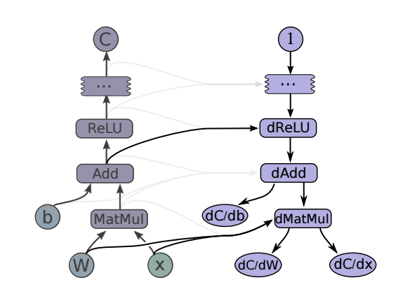
To compute the gradient in a neural network, we can use automatic differentiation, a technique to compute derivatives in computational graphs in a modular way. It is based on the chain rule, which says that the derivative of a composition of two functions and can be decomposed into . In a computational graph, we can compute the derivative of any edge with respect to any other edge by first computing the derivative of the last node and then compute the derivative of all the previous nodes by decomposing them in the same way. Derivatives are then passed backwards through the computational graph. An example is depicted in Figure 2.4.
2.1.2 Normalization
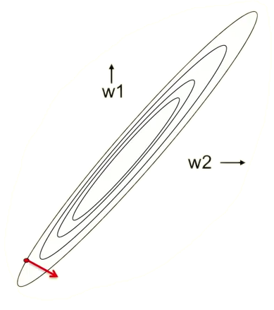
Neural network training is highly sensitive to the mean and variance of the data. They affect the cost, gradients, activations and the operation region of the activation functions. This issue makes it hard to select good learning rates, parameter initializations and to set other hyperparameters. Also, scale differences between dimensions within a dataset result in skewing the cost surfaces (Figure 2.5a), thus resulting in a wrong direction of the gradients. Normalizing the data to zero mean and unit variance alleviates these issues (Figure 2.5b). Furthermore, normalization is not only important for the network inputs and targets but also for the activations inside the network. During training, each layer has to constantly adapt to its changing input distribution caused by the optimization of the previous layers. For alleviating this issue, Ioffe and Szegedy [7] proposed batch normalization, a technique consisting in ensuring zero mean and unit variance for activations for each minibatch resulting in training time reduction by an order of magnitude.
In the next section we extend the discussion of deep learning techniques to reinforcement learning.
2.2 Reinforcement Learning
Reinforcement learning is concerned with learning through interaction with an environment. At every timestep, a learner or decision-maker called agent executes an action and the environment in turn yields a new observation and a reward, as shown in Figure 2.6. The task of the agent is to maximize the sum of rewards received during the interaction with the environment.
More formally, we can define a state as all the information the agent has about the environment at a given timestep. Generally, this information might not include the full state of the environment (e.g., in a card game the state would include the agent's hand but not all opponents' hands even though they are part of the full state of the game).
An action encodes how the agent can interact with the environment. The mapping from states to actions is called policy . A policy can either be stochastic (e.g., a probability distribution of actions over states) or deterministic.
The reward is a feedback informing the agent about the immediate quality of its actions. Typically, the function generating the rewards is defined by an expert and can depend on the last state and action . The reward signal can encode the goal of the agent at different levels. For instance, in chess the agent can be rewarded at each capture or only at the end of the match.
The goal of the agent is to maximize the sum of the rewards received by the environment, namely the return . The discount factor is to guarantee the convergence of the sum if the time horizon is not finite (infinite horizon). In the next section, we present a brief overview of classical approaches to solve reinforcement learning problems.
2.2.1 Learning Approaches
Reinforcement learning algorithms can be categorized as either value-based, policy-based or a combination of the two. Value-based methods consist in explicitly learning the value of all states and using it to select the action that leads to the highest-valued state. In this setting, the value function is defined as the expected return of the agent being in state and then following the policy , while the action-value function is defined as the expected return of the agent being in state , executing action and then following the policy . The advantage function connects both.
For deterministic policies, can be formulated recursively by the so-called Bellman equation
Knowing for each state-action pair, the best policy is to select the action with the highest action value at every timestep, i.e., . In practice we neither know nor in the first place. However, even when starting from a random , it is possible to iteratively update by exploiting the Bellman equation and to converge to (and therefore to ). This powerful approach is a key element in recent Deep-Q-Networks (DQN), which will be discussed further in Section 3.1.
In continuous action spaces, however, maximizing over is infeasible as there are infinite actions to consider. Even discretizing the action space becomes intractable for relatively low dimensional action spaces (curse of dimensionality). To overcome this issue, it might be better to directly learn a (parametrized) policy instead of a value function. Algorithms following this approach are called policy-based. One of the most successful class of policy-based algorithms is policy gradient [8, 9, 10]. Policy gradient approaches directly optimize the policy parameters by following the direction of the gradient of the expected return with respect to the policy parameters (), which can be directly estimated from samples.
A mixture of the value-based and policy-based approaches are actor-critic algorithms. These approaches make use of both a parametric policy (actor) and a value function estimator (critic), used to improve the policy. A very recent actor-critic approach for learning deterministic policies is Deterministic Policy Gradients (DPG) [11]. DPG uses a differentiable action-value function approximator to obtain the policy gradient by taking the derivative of its output with respect to the action input . The policy gradient is then computed as . Deep Deterministic Policy Gradient (DDPG), a DPG with neural network function approximators, will be discussed further in Section 3.2.
2.2.2 Exploration and Exploitation
One of the biggest issues in reinforcement learning is the tradeoff between exploration and exploitation. Acting greedily (exploitation) with respect to an approximated function (e.g., Q-function) and choosing the current best action might prevent the agent from discovering new better states and therefore prevent improvement of the policy. On the contrary, excessive exploration might slow down the learning or even results in harmful policies. A tradeoff is therefore necessary. Usually, noise is added to the actions during training. In the case of discrete actions, the -greedy policy is a common solution: the agent acts randomly with probability and greedily with probability . In the case of continuous actions, Gaussian noise could instead be added. In this thesis, we will use these simple strategies. However, the exploration-exploitation tradeoff is still an open problem in reinforcement learning. Alternative exploration strategies might consist in artificially rewarding exploration or even leaving the decision about exploration completely to the agent. We will come back to this topic in Section 6.2.
3 Deep Reinforcement Learning
As discussed in the previous section, reinforcement learning heavily relies on either approximating the Q-function (in the case of value-based algorithms) or on the policy parameterization (in the case of policy-based algorithms). In both cases, the use of rich function approximators or policies allows reinforcement learning to scale to complex problems. Neural networks have been successfully used as function approximators in supervised learning and are differentiable, a useful quality for many reinforcement learning algorithms. In this section, we focus on two recent reinforcement learning algorithms. The first one, Deep Q-Network (DQN) [1, 13], is a value-based algorithm successfully able to play 49 Atari games from pixels better than human experts. The second one, Deep Deterministic Policy Gradients (DDPG) [12], is an actor-critic algorithm, an extension to DQN for continuous actions.
3.1 Deep Q-Network (DQN)
DQN is a value-based algorithm using a neural network to approximate the optimal action-value of each action in a given state. The training targets for are computed via the Bellman equation . The network is trained to minimize the mean squared error with respect to the Q-function, i.e.,
However, the dependence of the Q targets on itself can lead to instabilities or even divergence during learning. Having a second set of network parameters , where LP is a low-pass filter (e.g., exponential moving average), stabilizes the learning.
Additional instabilities can arise from training directly on the incoming states and rewards, since, unlike supervised learning, the input data (state-action pairs) is highly correlated as they are part of a trajectory. Furthermore, the policy and therefore data distribution might change quickly as evolves. DQN solves both issues by storing all transitions in a replay memory dataset and then learning on minibatches consisting of random transitions from . This trick breaks the correlation of the input data and smoothes the changes in the input distribution. It also increases data efficiency by allowing the agent to perform multiple gradient descend steps on the same transition.
Finally, to ensure sufficient exploration, a simple -greedy policy, i.e., . This off-policy approach is possible because the algorithm does not learn on full trajectories but only on isolated transitions. The complete algorithm is shown in Algorithm 1.
3.2 Deep Deterministic Policy Gradient (DDPG)
As discussed in the introduction, a parametrized policy is advantageous for control because it allows for learning in continuous action spaces. Since DDPG is an actor-critic policy gradient algorithm, there is a policy network with parameters in addition to the action-value network with parameters .
The training targets for Q are computed as in DQN, with the only difference that now depends on . Using the mean squared error, we derive the cost function for Q
As the targets depend on the explicit policy network, we also need the target policy parameters . Here, LP will be an exponential moving average with update rule and .
The policy is trained via policy gradient
that is, is the cost function for
As actions are continuous, correlated Gaussian noise is added to the actions to ensure exploration. More specifically, , where is a normally distributed random variable and a hyperparameter controlling the frequency of the noise. Again, this off-policy approach is possible because the algorithm does not learn on trajectories but only on isolated transitions. Algorithm 2 shows the complete learning procedure.
4 Implementation
A big challenge in deep reinforcement learning implementations are efficient neural network routines. The most critical part are the inner products of inputs and weights and the respective derivatives in each layer. We first coded in MATLAB, a popular machine learning tool providing efficient linear algebra routines. Due to the lack of automatic differentiation, we implemented gradient propagation routines, as well as the RMSProp and ADAM optimizers. The code can be found on the CD of this thesis.
However, due to the high computational demands of neural networks, we also developed a TensorFlow implementation. TensorFlow [14] is an open source Python / C++ library providing fast routines ( times faster than MATLAB from our experience) for deep learning, accomplished through GPU support. It features automatic differentiation and therefore allows for much more flexible network and algorithm design. Additionally, TensorFlow provides a wide variety of built-in optimizers (e.g., ADAM) and operations (e.g., batch normalization). The results shown in this thesis have been produced by the TensorFlow implementation, which can be found on the CD of this thesis.
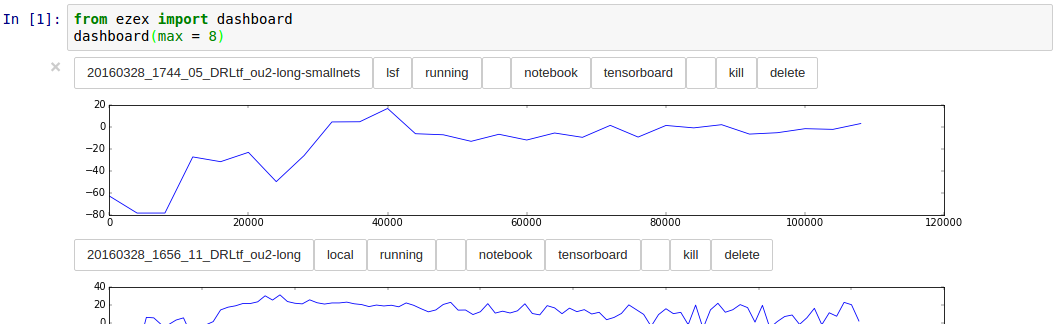
Another concern in setting up the testing framework regarded the ability to run several experiments on computing clusters with job schedulers while having a changing codebase. For this purpose, we wrote ezex, a small framework that provides basic operations (e.g., starting and aborting jobs) and a visualization of running and finished LSF (or SLURM) jobs via Jupyter Notebooks.
4.1 DDPG
Our DDPG implementation is as close as possible to the original paper. Its evaluation is performed on low-dimensional true state inputs and not on visual inputs due to time and software limitations. Figure 4.2 shows the layouts of the neural networks used, while Table 4.1 the hyperparameters used. The layers are initialized with small random weights.
| Hyperparameter | Value | Note |
|---|---|---|
| Minibatch size | 32 | |
| Policy learning rate | Step size for ADAM | |
| Critic learning rate | Step size for ADAM | |
| Policy weight decay | ||
| Critic weight decay | L2 cost for each parameter | |
| Target update rate | ||
| Replay memory size | Older transitions are discarded | |
| Exploration noise | 0.2 | |
| Exploration noise reversion rate | 0.15 | The overall noise variance is 0.13 |
| Reward discount | 0.99 | |
| Warm-up time | Timesteps until training starts |
4.2 The Cart-Pole Problem
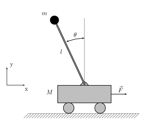
Although the final goal is to apply deep reinforcement learning in real-world settings (e.g., robotics), testing in these environments can be dangerous and expensive both in terms of money and human expert labor. Simulated environments are well suited for testing reinforcement learning systems extensively as the testing process is cheap and can be easily automated. For these reasons, both DQN and DDPG have been originally evaluated in simulated environments. In the original works DQN was tested on several Atari games using the simulator ALE [15], while DDPG has been evaluated in more than 20 physical environments using the MuJoCo [16] simulator. The authors showed that the algorithms and the same hyperparameters work on a wide variety of tasks without the need of hand-tuning them for each individual task. In our implementation, we also used MuJoCo but, because of time constraints, we evaluated DDPG only on the cart-pole (Figure 4.3), a standard reinforcement learning benchmark problem. The task is a standard non-linear control task. The goal is to indirectly swing-up and balance a pole placed on a cart by applying control force to the cart. Environment details (e.g., masses, friction coefficients, etc.) can be found in the MuJoCo model file cartpole.xml.
5 Evaluation
Even though DDPG turned out to be highly sensitive to the reward functions, they have not been included in the original paper. Among the several reward functions we tried, the most reliable one is
Here, has the highest influence, giving -1 when the pole is hanging down and 1 when it is standing up. The additional terms consist in penalties for the action , the cart position (for not being in the middle) and the rotation speed of the pole . However, we noticed that even slight changes to the parameters of the reward functions impaired the learning dramatically.
Below, we report results on varying the reward function and the hyperparameters. In particular, we evaluate the effects of batch normalization, experience replay and the use of a target network. All experiments have been averaged over ten trials.
5.1 Reference Results Without Batch Normalization
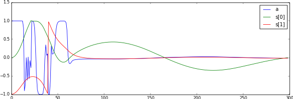
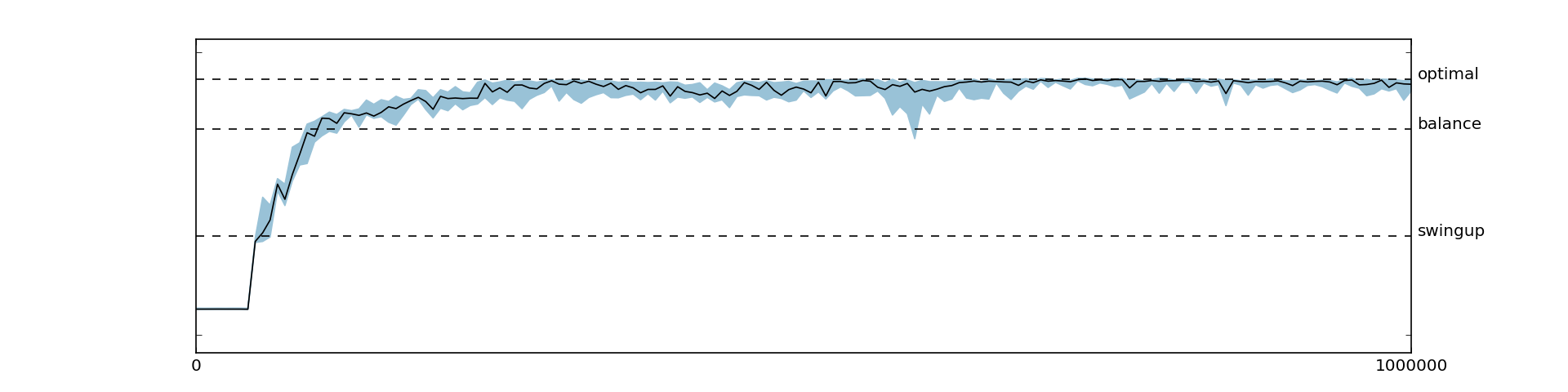
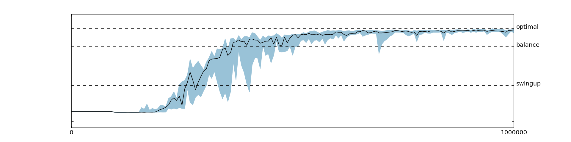
Here, we report the best results we achieved. The reward function used is the handcrafted one described above and we did not use batch normalization. With these settings, the agent was consistently able to learn the optimal swing-up and balance policy. The returns and some sample trajectories over the course of the learning process are depicted in Figure 5.1 and Figure 5.2, respectively.
We stress that, even though we used constant episode lengths, shifting the rewards (i.e., adding a constant) had an impact on the learning stability. At first we added a bias to ensure the returns for the initial policy were zero to match the initial values, but having a negative bias (introduced by ) improved the learning consistency significantly.
5.2 Applying Batch Normalization
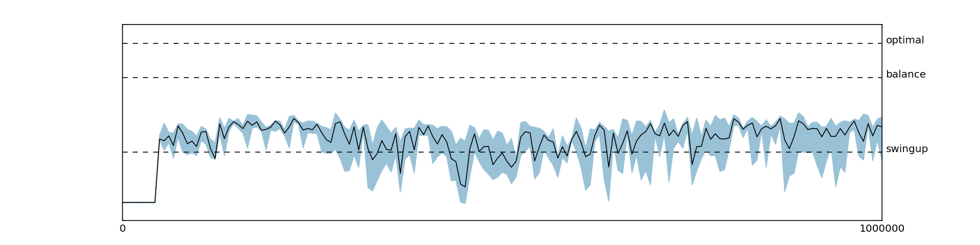
We then evaluated the same reward function with batch normalization. Surprisingly, we observed much worse results, as shown in Figure 5.3. Even though we tried the canonical as well as the non-standard batch normalization used in the DDPG paper, the agent was never able to balance after swinging up. This behavior might be due to the cart-pole environment, as the original paper also reported slightly inferior results for batch normalization on cart-pole. It could also be due to the fact that batch normalization introduces additional noise during learning. A very recent method claiming to alleviate this issue and that could be interesting for future research is weight normalization [17].
5.3 Disabling Target Network and Replay Memory
Consistent with the findings from the original paper, we observed reduced performance when disabling the target networks (Figure 5.4) or the replay memory (Figure 5.5).
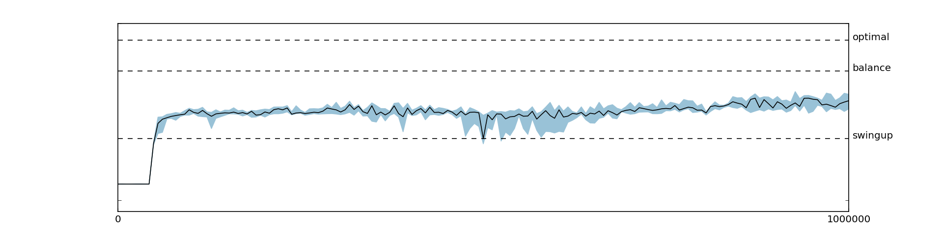
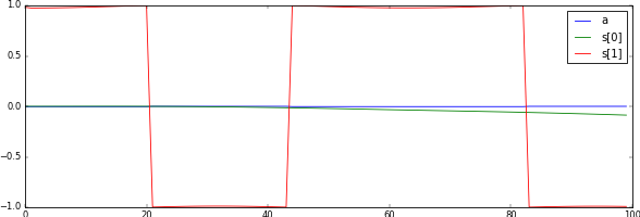
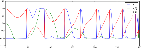
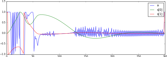
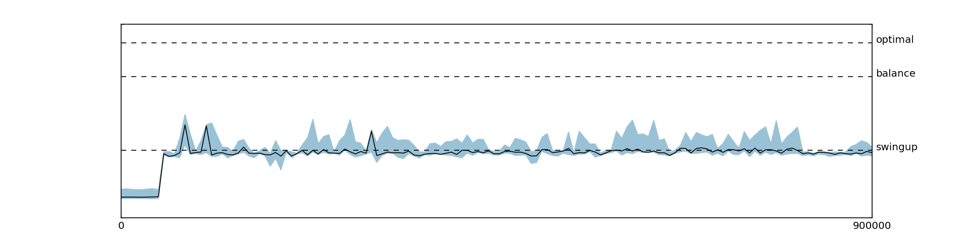
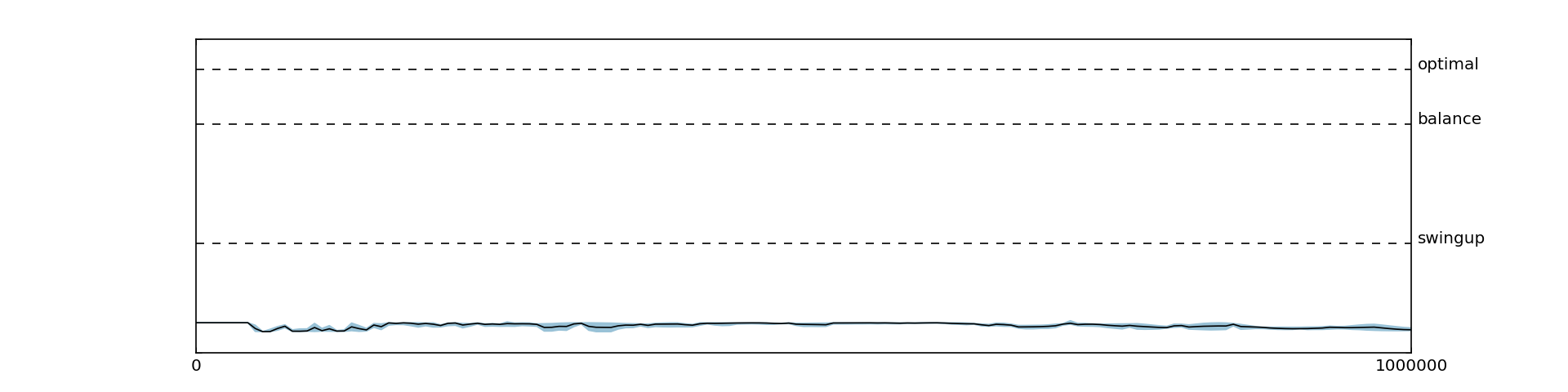
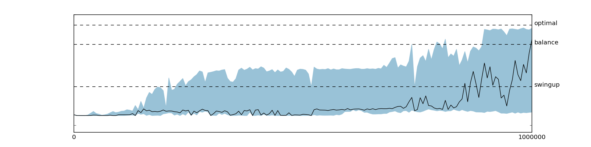
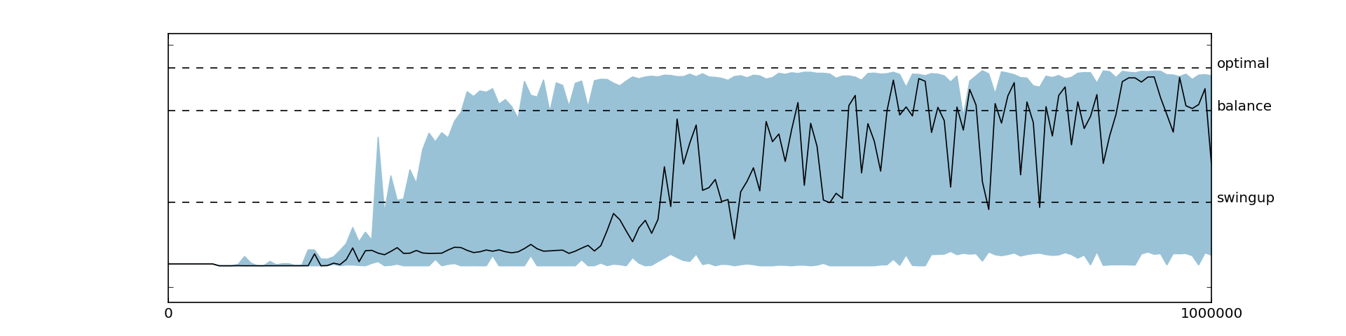
5.4 Sparse Reward Functions
As already discussed, we found DDPG to be very sensitive to the reward function. Initially, we were able to learn only with smooth reward functions, while using a sparse reward function encoding only the actual goal (i.e., rewarding the agent only when the pole is standing upright ), there was no improvement over the initial policy at all, as shown in Figure 5.6. At first, we thought that this behavior might be due to poor exploration of the state space and that the agent, never reaching the goal state, does not know where to get positive rewards. While this might in fact be an issue in more complicated environments, it was not the issue in the cart-pole. Instead, we found that increasing the magnitude of the reward and increasing the warm-up time helped the agent to learn good action value function and policy, as shown in Figures 5.7, 5.8 and 5.9. In general, extending the warm-up time stabilized learning tremendously. This behavior might be due to the fact that transitions from initially diverging policies have a lower chance to get sampled from the replay memory since the replay memory is already filled with many transitions from the warm-up time.
6 Conclusion and Future Work
With this thesis, we have provided an analysis of the state-of-the-art deep reinforcement learning algorithm DDPG. The results from the original papers have been reproduced and we successfully trained an agent for solving the cart-pole balance and swing-up tasks with continuous actions. We provided an analysis of the performance for sparse reward functions and evaluated the use of batch normalization, target network and replay memory.
We showed that DDPG was able to learn a non-trivial control policy, but there are several limitations that need to be solved before it will be possible to apply it to robotics. Below, we identify the major weaknesses and propose future avenues of research.
6.1 Data Efficiency
The first significant issue of deep reinforcement learning is data efficiency. In our test cases we experienced that in order to learn high-quality policies, the algorithm had to be fed with a high number of samples. Considering that real control problems are much harder than the simple task we evaluated, DDPG is not ready for real world problems.
There are, however, several papers improving DQN and some of the techniques proposed can be applied to DDPG with slight modifications. Prioritized experience replay [18] is for instance a technique for improving data efficiency by not sampling transitions uniformly from the replay memory but instead sampling according to the importance of a transition. Using the temporal difference error as a measure of importance, the authors achieved new state-of-the-art results on the DQN Atari benchmark games.
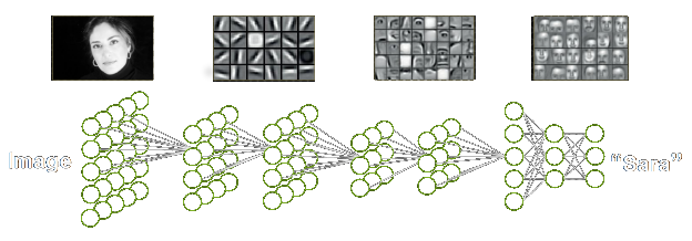
An alternative way to reduce the number of parameters (and therefore the number of required samples) is to move the first layers of the both the policy and the networks to a common preprocessing network , as shown in Figure 6.1. Since neurons in the first layers have to be useful to many other neurons in the following layers, they tend to learn task independent features anyway (e.g., for visual inputs these are typically edge filters as in Figure 2.3) and could therefore be combined in a single network. Such a network would then be trained by the gradients from both and . Having would also allow us to introduce additional function approximators for the value function or to learn model without much parameter overhead. Furthermore, learning a model and a value function could serve as a good regularizer for since transition data (model) and value data are currently unused in the DDPG framework.
Moreover the model and the value function can be used to estimate another policy gradient, since the expected return can be also expressed via . This approach is called value gradient. Because it assumes a deterministic model, it is only applicable in deterministic environments. However, there have been recent advances in expressing stochasticity in neural networks [19]. Building on this idea, Heess et al. [20] presented Stochastic Value Gradients, extending the value gradient approach to stochastic neural network models and policies. Even though these approaches have not been covered in this thesis, they seem a promising direction for further research.
6.2 Exploration
Another possible improvement to DDPG regards more efficient exploration. More specifically, stochastic policies that are able to encode multiple good actions instead of relying on -greedy exploration can speed up learning exponentially as Osband et al. [21] showed for DQN. As already mentioned in the introduction, rewarding exploration can be a way to enable the agent to actively explore. By learning a transition model for DQN and using the model error as a proxy for exploration (i.e., rewarding according to the model error) Stadie et al. [22] were able to improve performance especially where the original DQN performed poorly.
6.3 Imitation
In robotics, a simpler way to adopt complex behavior or to bootstrap the learning is imitation, consisting in using target trajectories for supervised learning of policies. In the case of DDPG, imitation could be employed by either initializing the networks by supervised training or by injecting target trajectories into the replay memory. For example, recently Silver et al. [2] were tremendously successful in the game of Go by first pre-training a policy network on human expert moves and subsequently improving it via reinforcement learning.
With regard to robotics, another helpful approach to avoid dangerous policies would be to initialize the Q-network with negative values for specific trajectories (e.g., for the violation of the joint limits).
6.4 Curriculum Learning
Curriculum learning [23] is a deep learning approach to learn complex functions by training on easier and more fundamental examples first and only gradually introducing more complicated examples. This could be also applied to reinforcement learning and especially robotics. For a robot the most fundamental concepts to learn are its own body dynamics and the skill to move without hurting itself. For example in table tennis, a robot could first learn to explore itself carefully (e.g., giving it rewards for exploration or punishing violation of joint limits) and subsequently learn striking movements and to win a match.
References
- Mnih, V., Kavukcuoglu, K., Silver, D., Rusu, A. A., Veness, J., Bellemare, M. G., Graves, A., Riedmiller, M., Fidjeland, A. K., Ostrovski, G., et al. (2015). Human-level control through deep reinforcement learning. Nature, 518(7540), 529–533.
- Silver, D., Huang, A., Maddison, C. J., Guez, A., Sifre, L., van den Driessche, G., Schrittwieser, J., Antonoglou, I., Panneershelvam, V., Lanctot, M., et al. (2016). Mastering the game of Go with deep neural networks and tree search. Nature, 529(7587), 484–489.
- Ng, A. Y., Coates, A., Diel, M., Ganapathi, V., Schulte, J., Tse, B., Berger, E., and Liang, E. (2006). Autonomous inverted helicopter flight via reinforcement learning. In Experimental Robotics IX, 363–372. Springer.
- Rosenblatt, F. (1958). The perceptron: a probabilistic model for information storage and organization in the brain. Psychological Review, 65(6), 386.
- Krizhevsky, A., Sutskever, I., and Hinton, G. E. (2012). ImageNet classification with deep convolutional neural networks. In Advances in Neural Information Processing Systems 25, 1097–1105.
- Kingma, D., and Ba, J. (2014). Adam: A method for stochastic optimization. arXiv preprint arXiv:1412.6980.
- Ioffe, S., and Szegedy, C. (2015). Batch normalization: accelerating deep network training by reducing internal covariate shift. arXiv preprint arXiv:1502.03167.
- Williams, R. J. (1992). Simple statistical gradient-following algorithms for connectionist reinforcement learning. Machine Learning, 8(3-4), 229–256.
- Baxter, J., and Bartlett, P. L. (2000). Direct gradient-based reinforcement learning. In Proceedings of the IEEE International Symposium on Circuits and Systems (ISCAS), 3, 271–274.
- Amari, S.-I. (1998). Natural gradient works efficiently in learning. Neural Computation, 10(2), 251–276.
- Silver, D., Lever, G., Heess, N., Degris, T., Wierstra, D., and Riedmiller, M. (2014). Deterministic policy gradient algorithms. In ICML.
- Lillicrap, T. P., Hunt, J. J., Pritzel, A., Heess, N., Erez, T., Tassa, Y., Silver, D., and Wierstra, D. (2015). Continuous control with deep reinforcement learning. arXiv preprint arXiv:1509.02971.
- Mnih, V., Kavukcuoglu, K., Silver, D., Graves, A., Antonoglou, I., Wierstra, D., and Riedmiller, M. (2013). Playing Atari with deep reinforcement learning. arXiv preprint arXiv:1312.5602.
- Abadi, M., Agarwal, A., Barham, P., Brevdo, E., Chen, Z., Citro, C., Corrado, G. S., Davis, A., Dean, J., Devin, M., et al. (2015). TensorFlow: large-scale machine learning on heterogeneous systems. Software available from tensorflow.org.
- Bellemare, M. G., Naddaf, Y., Veness, J., and Bowling, M. (2013). The arcade learning environment: an evaluation platform for general agents. Journal of Artificial Intelligence Research, 47, 253–279.
- Todorov, E., Erez, T., and Tassa, Y. (2012). MuJoCo: a physics engine for model-based control. In Proceedings of IROS 2012, 5026–5033. IEEE.
- Salimans, T., and Kingma, D. P. (2016). Weight normalization: a simple reparameterization to accelerate training of deep neural networks. arXiv preprint arXiv:1602.07868.
- Schaul, T., Quan, J., Antonoglou, I., and Silver, D. (2015). Prioritized experience replay. arXiv preprint arXiv:1511.05952.
- Kingma, D. P., and Welling, M. (2013). Auto-encoding variational Bayes. arXiv preprint arXiv:1312.6114.
- Heess, N., Wayne, G., Silver, D., Lillicrap, T., Erez, T., and Tassa, Y. (2015). Learning continuous control policies by stochastic value gradients. In Advances in Neural Information Processing Systems, 2926–2934.
- Osband, I., Blundell, C., Pritzel, A., and Van Roy, B. (2016). Deep exploration via bootstrapped DQN. arXiv preprint arXiv:1602.04621.
- Stadie, B. C., Levine, S., and Abbeel, P. (2015). Incentivizing exploration in reinforcement learning with deep predictive models. arXiv preprint arXiv:1507.00814.
- Bengio, Y., Louradour, J., Collobert, R., and Weston, J. (2009). Curriculum learning. In Proceedings of the 26th Annual International Conference on Machine Learning, 41–48. ACM.